Same Dynamics, Different Structures in Energy‑Preserving Operator Fits
| $c^{1}_{23}$ | $c^{2}_{31}$ | $c^{3}_{12}$ | |
|---|---|---|---|
| $c$ | 1.000 | 1.000 | 1.000 |
| $c+t\,g_A$ | — | — | — |
coefficient change —
max field difference —
max trajectory difference —
forced ceiling of any gauge-blind fit (Corollary 1) —
Abstract
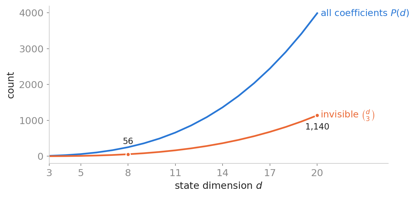
Models $\dot z=J(z)\nabla E(z)$ with skew-symmetric $J$ affine in the state and quadratic $E$ are fitted to trajectories because they conserve energy by construction. The fit determines the dynamics without determining the coefficients: in dimension $d$, for any quadratic energy with invertible Hessian, the coefficient changes leaving the vector field untouched at every state form a subspace of dimension $\binom{d}{3}$, known in closed form before any data are collected: 56 of the 224 bracket coefficients at $d=8$. Its dimension recurs at two reduced orders of a model-reduction benchmark, and on five of thirteen algebras it contains a non-isomorphic Lie algebra reproducing the field, trajectories and Jacobi identity to machine precision, so no residual or conservation diagnostic detects the substitution. A certificate computed from a hypothesized bracket and the energy alone decides in advance which of two levers restores identifiability; over thirteen algebras, its routing matched the measured outcome on all nine where both levers were run. Where it permits, a Levenberg–Marquardt retraction along the invisible directions recovers the coefficients in 8–9 steps without moving what the data determined, at two orders of magnitude less work than the penalty and constrained-solver arms that also recover them; where it does not, a second experiment with pairwise-distinct curvature ratios raises the fitted-to-true coefficient cosine from 0.336 to 1.0000, while a proportional second energy at the same cost gains nothing.
The failure, measured
On $\mathfrak{su}(3)$ the rollout error falls from $0.14$–$0.28$ at eight orbits to $2$–$6\cdot10^{-3}$ at $512$, while from $128$ orbits on the cosine stops at $0.2355$–$0.3094$, within $10^{-4}$ of the ceilings computed from each draw's energy. The $64\times$ budget increase improves prediction by a factor of $29$ to $67$ across the three draws and moves identification only to its precomputed ceiling. The rigid body behaves the same: its cosine stays within $1.2\cdot10^{-4}$ of its per-draw ceilings ($0.2620$/$0.2523$/$0.3347$) at every budget. The cap is a property of the estimator's reach, not of the truth: on these three draws the $56$-dimensional invisible subspace counted below holds between $0.951$ and $0.972$ of the true $\mathfrak{su}(3)$ structure-constant norm, the complement of those ceilings, and the solve returns the one coset representative with no component in it. The fraction is a property of the draw, and other draws give other values.
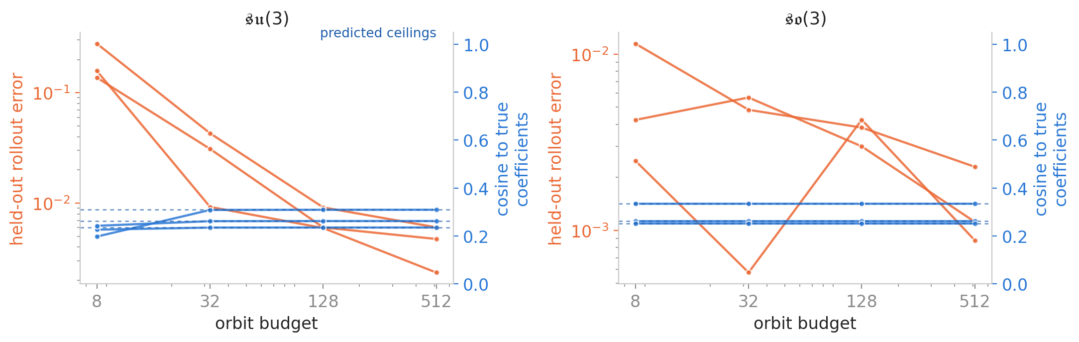
When $A$ is unknown, the energy must be co-estimated with the bracket; we alternate least squares over $(J_0,c)$ and the energy parameters $\theta$, at ridge $3\cdot10^{-3}$. Co-estimation leaves the split of overall scale between $c$ and $\theta$ undetermined, which the cosine is blind to: it normalizes both arguments and is reported in absolute value. On the same grid it scatters from $0.565$ to $1.000$ at $d=3$ and $0.001$ to $0.102$ at $d=8$, with no trend in budget: no longer confined to a fixed complement of the gauge, the fit lands on an arbitrary representative of a larger solution set. A cosine of $0.003$ in $\R^{224}$ is a factor of roughly $18$ below the $0.053$ two independent random unit vectors average in absolute value. A cosine of $1.00$ at $d=3$ is the same arbitrariness with better luck; neither number measures recovery.
The unidentifiable subspace
Theorem 1 (The gauge). Let $A$ be symmetric and invertible. Then \[ \ker\Phi_A=0\oplus K_A,\qquad K_A=\bigl\{c:\;c^k_{ij}=\textstyle\sum_m A_{km}\,g_{mij},\;g\in\Lambda^3\mathbb{R}^d\bigr\}, \] where $\Lambda^3\mathbb{R}^d$ is the space of $3$-tensors changing sign under every transposition of their slots. Consequently $J_0$ is identifiable and, for every invertible $A$, $\dim K_A=\binom{d}{3}$ and $\operatorname{rank}\Phi_A=\tfrac{d(d-1)}{2}+\tfrac{d(d^2-1)}{3}$.
Of the 252 bracket parameters at $d=8$ the design sees 196; the remaining 56, or 22%, leave the vector field pointwise unchanged. They span the kernel of the parameters-to-dynamics map, so no optimizer, no regularizer, and no additional trajectory removes them, and that kernel depends only on the state dimension and the energy Hessian, available in closed form before a single measurement is taken.
The two integers of Theorem 1 are measured by SVD of the design matrix at generic $\mathcal N(0,I)$ states for $d\in\{3,5,6,7,8,9,10,12\}$. Predicted and measured agree on every row, with fifteen orders of magnitude between the smallest retained and the largest discarded singular value, so the rank decision is not a tolerance choice, and the $J_0$-block contributes nullity $0$ throughout. The number of invisible directions is $\binom d3$ for every invertible $A$: measured at $d=6$ and $d=8$ for diagonal SPD, dense SPD and generic invertible non-symmetric $A$, the nullities are $20,20,20$ and $56,56,56$ — anisotropy re-aims the invisible subspace without resizing it, and no single quadratic energy reduces it. At corank one the kernel collapses to $\binom d3$, the invertible value $20$ and $56$, and it grows only from corank two, to $23$ and $67$.
Two conditions, not one, make $\dot z=J(z)\nabla E(z)$ a Poisson system: the degree-one part of the cyclic sum is the Jacobi identity on $c$, and the degree-zero part says $J_0$ is a scalar two-cocycle of the algebra $c$. An arbitrary skew $J_0$ does not satisfy it: paired with the $\mathfrak{su}(3)$ constants, a generic one leaves a residual of $27.8$ where the degree-one part sits at $5\cdot10^{-16}$, and only $8$ of the $28$ skew parameters are compatible, the coboundaries produced by recentering, as Whitehead's lemma requires for a semisimple algebra.
Conversely, for $E=\tfrac12\|z\|^2+\tfrac13\sum_l g_l z_l^3$ with all $g_l\ne0$ the measured nullity is $0$ at $d\in\{6,8\}$, for a diagonal and for a generic symmetric cubic: a nonlinear energy removes the gauge outright at this bracket degree.
The forced ceiling
Corollary 1 (Spherical-top degeneracy and the forced ceiling). For a compact semisimple Lie algebra expressed in a basis orthonormal for the negative Killing form, the isotropic energy $E=\tfrac12\|z\|^2$ is the quadratic Casimir and the Lie–Poisson field vanishes identically (the spherical top in $d$ dimensions). Let noiseless field data come from $(J_0^\ast,c^\ast)$ under $E=\tfrac12z^{\!\top}\!Az$ with $A$ invertible, at sufficiently many states in general position, and $(\hat J_0,\hat c)$ the minimum-norm least-squares estimate in the Frobenius inner product. Then \[ \hat J_0=J_0^\ast,\quad \hat c=P_{\KA^\perp}c^\ast,\quad \cos(\hat c,c^\ast)=\frac{\|P_{\KA^\perp}c^\ast\|}{\|c^\ast\|}, \] a number computable before data collection, which also upper-bounds $\cos(\hat c,c^\ast)$ for any estimator returning an element of $\KA^\perp$. If $c^\ast$ are the constants of a compact semisimple algebra in a Killing-orthonormal basis and $A=I$, the spherical top, that ratio is $0$: the estimate itself vanishes, so no such estimator recovers any component of $c^\ast$, and the cosine is undefined there rather than small. The qualifier is on the basis: total antisymmetry is a property of the presentation, not of the algebra.
The rigid body makes the ceiling concrete. With $c^\ast=\varepsilon$ and $A=\operatorname{diag}(a)$, $a_k=1/I_k$, the gauge is the single direction $a\odot\varepsilon$, and the three inner products $\|\varepsilon\|^2=6$, $\|a\odot\varepsilon\|^2=2\sum_ka_k^2$ and $\langle\varepsilon,a\odot\varepsilon\rangle=2\sum_ka_k$ give \[ \cos(\hat c,\varepsilon)\;=\;\Bigl(\,1-\bigl(\textstyle\sum_k I_k^{-1}\bigr)^2\big/ \bigl(3\textstyle\sum_k I_k^{-2}\bigr)\Bigr)^{1/2}. \] By Cauchy–Schwarz the fraction is at most $1$, with equality if and only if the moments of inertia are equal, so the ceiling vanishes precisely for the spherical top and grows with asymmetry.
Corollary 1 predicts, before any data are collected, the cosine a gauge-blind least-squares fit reports against the true structure constants. Predicted and measured agree to six digits in three cells: $0.598200$ for a mixed truth under $A=I$, $0.156128$ for $\mathfrak{su}(3)$ under a diagonal $A$ at $d=8$, and $0.420560$ for the $\mathfrak{so}(3)$ rigid body with inertia $(1,2,3)$ — the system running in Figure 1. In the recovery experiments the same agreement holds cell by cell to $|\Delta|\le5.6\cdot10^{-17}$ over five energy draws.
The gauge on community benchmark data
Every system above is hand-built, but the same computation runs on data we did not generate: the 2D Burgers snapshots published with Gkimisis et al. A POD basis is orthonormal, so the reduced energy is isotropic, $A=I$, and the reduced quadratic operator is the $c$-block of the model.
At $r=5$ and $r=8$ the measured nullity equals $\binom r3$; at $r\ge10$ the count exceeds the prediction and the gap at the cut falls to $1.02$, so no tolerance turns it into an integer. Two controls localize the excess: at matched sample count, generic Gaussian states return $\binom r3$ at every order, as do Gaussian states whose per-coordinate scales match the decaying POD amplitudes, ruling out amplitude anisotropy. What remains is the configuration of the trajectory's states; these snapshots, a single decaying solution, sit in the sampling lemma's exceptional set at $r\ge10$. At the orders a practitioner would choose here, $r$ between $10$ and $20$, the basis already capturing $99.98\%$ of the snapshot energy, one simulation does not expose the gauge as an integer.
| $r$ | $\binom r3$ | nullity (Burgers) | gap | nullity (generic) | gap | POD energy |
|---|---|---|---|---|---|---|
| 5 | 10 | 10 | $4.4\cdot10^{12}$ | 10 | $1.3\cdot10^{15}$ | 0.9958 |
| 8 | 56 | 56 | $5.3\cdot10^{8}$ | 56 | $3.8\cdot10^{14}$ | 0.9993 |
| 10 | 120 | 121 | 1.10 | 120 | $2.2\cdot10^{14}$ | 0.9998 |
| 15 | 455 | 704 | 1.02 | 455 | $1.2\cdot10^{14}$ | 1.0000 |
| 20 | 1140 | 2089 | 1.02 | 1140 | $6.7\cdot10^{13}$ | 1.0000 |
Table 1. The gauge on the 2D Burgers snapshots of Gkimisis et al., against generic Gaussian states at matched sample count. “Gap” is the ratio of the singular values either side of the rank cut; a reported dimension is read as an integer only above about $10^4$.
The closed-form gauge basis lies in the kernel of the sampled design to $9\cdot10^{-18}$ relative, so arbitrary gauge displacements separate admissible fits: adding to the minimum-norm fit a gauge element of norm $0.24\|\hat c\|$ at $r=5$ and $0.68\|\hat c\|$ at $r=8$ changes the generated field by $1.2\cdot10^{-16}$ and $6.2\cdot10^{-14}$. Two codes fitting these snapshots under different conventions for the free entries can disagree about two-thirds of the operator and remain indistinguishable from the data. The fitted operator is not a Lie bracket: its scale-normalized Jacobi residual is $0.51$ at $r=5$ and $0.41$ at $r=8$, against the dimension-aware gate at $3\cdot10^{-5}$ and $10^{-5}$. Theorem 1 nowhere uses the Jacobi identity and applies to this operator unchanged.
When the invisible directions cross isomorphism classes
Motion along the kernel also changes the bracket's isomorphism class, the algebra's identity up to a change of basis. On five algebras of the thirteen-algebra battery, one indecomposable and nilpotent at $d=4$, a Lie algebra not isomorphic to the truth reproduces the true vector field to $7.7\cdot10^{-15}$ over 3000 states and its RK4 trajectories to $7.8\cdot10^{-16}$ over 300 steps, at Jacobi residual at most $1.2\cdot10^{-16}$. Such a model passes every check a practitioner would run, conservation included: nothing in the data distinguishes it from the truth, and the two disagree on the algebra's invariants.
Could impersonation be a low-dimensional accident? At $d=3$ every unimodular linear Poisson structure on $\mathbb R^3$ is $\nabla C\times\cdot$, the one-dimensional gauge merely rescales the Casimir, and the resulting family moves through the classical Bianchi types. The claim therefore rests on the $d=4$ rows, specifically the indecomposable $\mathfrak n_4$: adding the invisible direction leaves the field, the Jacobi residual and the $300$-step trajectories agreeing to $10^{-15}$ or better while moving both the Killing signature and the derived-algebra dimension, from $(0,4,0)/2/1$ to $(0,1,3)/3/1$, and between $65\%$ and $88\%$ of the direction lies outside $B^2$ across the three energy draws, so the motion is no change of basis in disguise.
Invisibility and variety membership degrade with $t$ as the polarization identity $\mathrm{Jac}(f+th)=t^2\mathrm{Jac}(h)$ predicts: on the four rows where $\mathrm{Jac}(h)$ sits above floating-point noise the measured residuals at $t=0.5$ and $t=1.0$ are $25$ and $100$ times those at $t=0.1$, all remaining at floating-point noise.
The certificate
Exact linear algebra on the pair (hypothesized bracket, energy), computed without trajectory data, decides which repair applies: $r_{\mathrm{Jac}}$ routes between the two levers, a constraint (the Jacobi identity) or a further experiment (a second energy); and its image in cohomology, $\iota_H$, separates fits that merely re-label the truth from fits that land on a different algebra. On the nine algebras where both levers were run the routing matched the measured outcome on every one, and the pair is strictly finer than the classical deformation invariant $H^2$, which misroutes three rows of the battery.
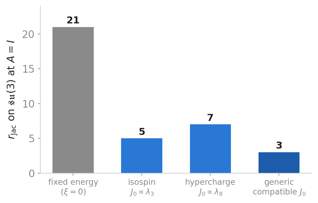
It is also not a function of the algebra alone: the energy enters through $\KA$, which $H^2$ ignores. Measured, $Z^2\cap\KA$ is $21$-dimensional for $\mathfrak{su}(3)$ at the isotropic energy ($A=I$) and $0$ at every anisotropic draw, with $H^2=0$ throughout.
| algebra | $d$ | $\dim K_A$ | $\dim H^2$ | $r_{\mathrm{Jac}}$ | $\iota_H$ | certificate route |
|---|---|---|---|---|---|---|
| $\mathfrak{so}(3)$ | 3 | 1 | 0 | 1 | 0 | second energy; re-labeling only |
| $\mathfrak{so}(4)$ | 6 | 20 | 0 | 2 | 0 | second energy; re-labeling only |
| $\mathfrak{su}(3)$ | 8 | 56 | 0 | 0 | 0 | Jacobi retraction recovers |
| $\mathfrak{sl}(2,\mathbb{R})$ | 3 | 1 | 0 | 1 | 0 | second energy; re-labeling only |
| $\mathfrak{se}(2)$ | 3 | 1 | 2 | 1 | 1 | non-isomorphic substitute verified |
| $\mathfrak{h}_3$ | 3 | 1 | 5 | 1 | 1 | non-isomorphic substitute verified |
| $\mathfrak{e}(3)$ (heavy top) | 6 | 20 | 1 | 0 | 0 | Jacobi retraction recovers |
| $\mathfrak{n}_4$ (filiform) | 4 | 4 | 6 | 1 | 1 | non-isomorphic substitute verified |
| $\mathfrak{h}_3\oplus\mathbb{R}$ | 4 | 4 | 13 | 2 | 2 | non-isomorphic substitute verified |
| $\mathfrak{se}(2)\oplus\mathbb{R}$ | 4 | 4 | 5 | 1 | 1 | non-isomorphic substitute verified |
| $\mathfrak{h}_5$ | 5 | 10 | 20 | 0 | 0 | Jacobi retraction recovers |
| $\mathfrak{n}_5$ (filiform) | 5 | 10 | 8 | 0 | 0 | Jacobi retraction recovers |
| $\mathfrak{aff}(1)\oplus\mathfrak{aff}(1)$ | 4 | 4 | 0 | 0 | 0 | Jacobi retraction recovers |
Table 2. The thirteen-algebra battery. $r_{\mathrm{Jac}}$ routes between the two levers and $\iota_H$ grades what the ambiguity costs: a change of basis at $\iota_H=0$, a non-isomorphic algebra at $\iota_H>0$. The rows with $\dim H^2>0$ but $r_{\mathrm{Jac}}=0$ — $\mathfrak{e}(3)$, $\mathfrak{h}_5$, $\mathfrak{n}_5$ — are the three the classical invariant misroutes.
The cheapest proxy rule, “nilpotent algebras impersonate”, is false: $\mathfrak h_5$ and $\mathfrak n_5$ are nilpotent at $d=5$ with $H^2=20$ and $H^2=8$ respectively, and both have $\rJac=\iotaH=0$: the retraction identifies them. Nor does $H^2$ order the rows, since $\mathfrak h_3\oplus\mathbb R$ has $H^2=13$ and impersonates while $\mathfrak h_5$ has $H^2=20$ and does not. In Table 2, $\iota_H$ is the only column separating the recoverable rows from the impersonating ones: zero on all eight of the former, positive on all five of the latter.
On the three reparameterization rows the verdict is a demonstrated isomorphism rather than an absence of detected change. On $\mathfrak{so}(3)$'s invisible line the motion rescales the slices, and a diagonal change of basis $S=\operatorname{diag}(\lambda)$ with $\lambda_k=\sqrt{\mu_i\mu_j}$ reproduces $f+th$ to $2\cdot10^{-16}$ at $t=0.1$, $0.5$ and $1.0$ without preserving the energy: $\|S^{\!\top}\!AS-A\|/\|A\|$ is $0.21$, $1.26$ and $3.00$ at those displacements. Those verdicts do not extend along the whole invisible line: at $t=-0.55$ under one fixed energy draw the algebra on $\mathfrak{so}(3)$'s line carries the Killing signature $(2,0,1)$ of $\mathfrak{sl}(2,\mathbb R)$ while still generating the identical field with the Jacobi identity intact, at field difference $1.4\cdot10^{-15}$. This is why every row with nonzero intersection routes to the energy lever regardless of $\iotaH$: motion along the gauge is a change of basis near the truth and not in the large.
The supplement carries the certificate to the pair $(J_0,c)$, one further linear block that never loosens the test: vacuous at $d=3$, it cuts the count at $\mathfrak{su}(3)$, $A=I$, from $21$ to $3$ for generic compatible $J_0$, rising to $5$ and $7$ exactly on the isospin and hypercharge strata. For compact semisimple $\g$ in a Killing-orthonormal basis at $A=I$, $Z^2\cap K_I$ is the space of closed Chevalley–Eilenberg $3$-cochains and $\rJac=d(d-3)/2+\nu$ with $\nu$ the number of simple factors — verified at seven of seven algebras; at $\mathfrak{su}(3)$ this is $20+1=21$. The drop is specific to the isotropic energy: at a generic anisotropic $A$ the intersection is already empty and the extension has nothing left to cut.
The intersection law
Theorem 2 (Intersection law). Let $A=\operatorname{diag}(a)$ and $B=\operatorname{diag}(b)$ be invertible, set $r_k=a_k/b_k$, and let $L_1,\dots,L_\ell$ be the level sets of $r$ (the groups of coordinates sharing a ratio). Then $K_A\cap K_B$ is spanned by the $a\odot e^\tau$ with $\tau$ a $3$-element subset of a single level set, where $e^\tau$ is the elementary totally antisymmetric tensor on $\tau$ and $(a\odot e)^k_{ij}=a_ke_{kij}$, so \[ \dim\bigl(K_A\cap K_B\bigr)=\sum_{t=1}^{\ell}\binom{|L_t|}{3}. \] In particular $b\propto a$ leaves the gauge at $\binom{d}{3}$, and pairwise distinct ratios annihilate it.
Group the $d$ curvature ratios $r_k=a_k/b_k$ into level sets (click a circle to move it between groups):
Theorem 2, evaluated live: equal colors share a ratio; each level set of size $s$ contributes $\binom{s}{3}$ surviving invisible directions.
The intersection law is tested on $\mathfrak{su}(3)$ at $d=8$ under a matched total budget of $16$ RK4 orbits of $24$ states, split evenly across each arm's energies, the structure constants solved blind by minimum-norm least squares. One anisotropic energy returns cosine $0.335838763882721$, the ceiling $0.3358387633$ predicted for that curvature vector, agreeing to eight significant digits. Partial ties and pairwise distinct ratios lift the recovery as the kernel dimension falls. The control arm, $B=2A$, gives two energy functions and two trajectory sets at the same total number of states but identical curvature ratios, hence a predicted intersection of $56$, the full gauge, and a measured recovery matching the single-energy arm to twelve significant digits. Data volume and energy count are thereby excluded, leaving the ratio spectrum, as Theorem 2 says.
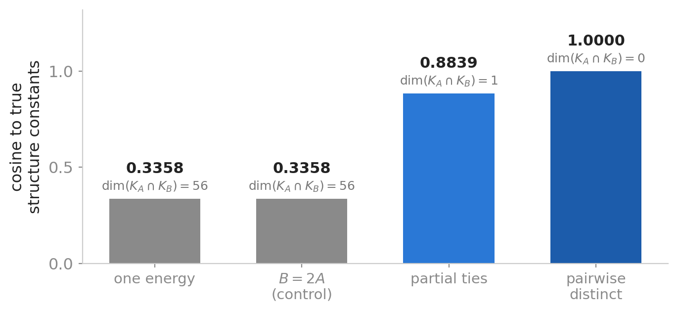
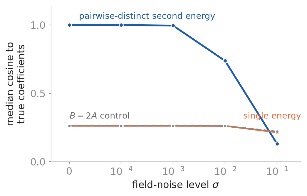
The ladder exercises the intersection law on noiseless fields; that is a statement about kernels and says nothing about conditioning, which is what decides whether the directions a second energy exposes arrive at a usable accuracy. Repeating the three arms at a fixed total row budget over five noise levels separates the two claims. The distinct arm gains its empty kernel at a quotient margin one to two orders of magnitude smaller, $4.2\cdot10^{-6}$ against $4.6\cdot10^{-4}$ on the first draw, so its recovery degrades faster: the lever leads by a wide margin through $\sigma=10^{-2}$ and loses at $10^{-1}$, and the budget rule prices the trade in advance from the stacked design: at $\sigma=10^{-3}$ it predicts $1.97\cdot10^{-1}$ against a measured $2.03\cdot10^{-1}$.
The Jacobi lever
The repair is a Levenberg–Marquardt retraction moving only inside the invisible coset $\hat c+K_A$, minimizing the Jacobi residual. Because every step lies in $K_A$, the retraction cannot change the fit to the data. On noiseless data from a single anisotropic energy and 16 orbits of 24 states, the retraction reaches cosine 1.0000 in 8–9 steps at Jacobi residual $1.6$–$2.5\cdot10^{-16}$. The standard alternative, a soft Jacobi penalty added to the loss with its weight tuned over $\lambda\in\{0.01,0.1,1,10\}$, also reaches 1.0000 but needs 1506–2440 steps and stops at residual $1.1\cdot10^{-9}$–$4.6\cdot10^{-8}$. On noiseless data the retraction therefore gains two to three orders of magnitude in iteration count and seven in certificate quality, and no accuracy.
The obvious alternative fails structurally. Minimum-norm Newton projection onto $\{\mathrm{Jac}=0\}$ always has the radial direction available, since $\mathrm{DJac}(c)[c]=2\,\mathrm{Jac}(c)$, so its steps flow down the homogeneous cone toward the abelian bracket $c=0$, halving the scale at each step. Measured, it terminates at a Jacobi residual of $1.0\cdot10^{-10}$, a diagnostic that looks conclusive, with the cosine stuck at $0.3454$ and the data residual at $0.863$: the fit to the observations is destroyed. The comparison is repeated against two solvers built for the job. One of them succeeds: on $\mathfrak{su}(3)$ the augmented Lagrangian also reaches cosine $1.0000$. What separates the methods is what they do to the component the data determined. The retraction is confined to $\KA$, so it cannot move that component and does not, displacing it by $7\cdot10^{-15}$ relative; the augmented Lagrangian moves it by $5.9\cdot10^{-6}$ and the soft penalty by $5.4\cdot10^{-6}$, both paying seven hundred to two thousand function evaluations against the retraction's eight. At a Lie point the constraint Jacobian is rank deficient by construction, its kernel being the coboundary space, and scipy's trust-region method reports that degeneracy before driving the quotient error to $1.0$, returning a bracket that satisfies the Jacobi identity and has no relation to the data; SLSQP terminates at its starting point.
Under noise a strongly weighted soft penalty does better. Swept over six decades, the penalty selects $\lambda\in[10^2,10^3]$ and reaches a $c$-cosine of $1.0000$ on every cell, a certificate of $8.0\cdot10^{-7}$, and a quotient error of $0.00110$, six times smaller than the $0.00705$ the retraction inherits from least squares. Jacobi constrains the identifiable component as well as the invisible one, so enforcing it in the full parameter space corrects part of the noise in what the data measured. The retraction cannot and is not meant to: moving only inside $\KA$ is what makes its guarantee unconditional and its cost ten steps against the penalty's median $609$ iterations.
The certificate under noise
Both integers the certificate reads come from tolerance cuts: a relative singular value below $10^{-10}$ counts as zero, a principal-angle cosine above $1-10^{-8}$ counts as an intersection. Those numbers are right at an exact Lie bracket and wrong at a candidate fitted to noisy data, the only place the test is ever applied. On $\mathfrak{su}(3)$ at $\sigma=10^{-3}$ the whole kernel lifts above the singular-value cut and its reported dimension falls from $56$ to $0$; on $\mathfrak{so}(3)$ the dimension survives but the kernel has rotated, and the reported intersection falls from $1$ to $0$. Both failures report $\rJac=0$, and $\rJac=0$ is what licenses the Jacobi lever, so the error runs the unsafe way: across a grid of four algebras, five noise levels and three seeds, the exact tolerances give the wrong count on $22$ of $60$ cells and all $22$ read zero where the truth is positive. Tying both cuts to the predicted relative quotient error removes the systematic part, and the implementation reports an integer only when the cut separates the two clusters by a factor of $10^2$, the smallest decade at which no wrong count survives on that grid, and otherwise refuses and routes to the second energy. Refusing is not a weaker answer: the second energy does not depend on the candidate reading.
| required margin $M$ | certified | wrong among them | refused |
|---|---|---|---|
| $10^{0}$ | 60 | 7 | 0 |
| $10^{1}$ | 51 | 3 | 9 |
| $10^{2}$ ← shipped | 43 | 0 | 17 |
| $10^{3}$ | 42 | 0 | 18 |
| $10^{4}$ | 38 | 0 | 22 |
| $10^{5}$ | 28 | 0 | 32 |
Table 3. The certificate re-read at a retracted candidate, over four algebras of known $\rJac$, five noise levels and three seeds. The exact tolerances get 22 of 60 cells wrong, all toward $\rJac=0$. The chosen $M=10^2$ is the smallest decade certifying nothing false on this sweep, so it is calibrated in sample rather than validated on held-out algebras.
Acceptance tests the recovered bracket twice: the scale-normalized residual must fall below a threshold, and the certificate re-evaluated at the recovered bracket must vanish. The threshold must be noise-aware: on noiseless data the retraction reaches $10^{-16}$ and a fixed $10^{-8}$ is the right test, but observation noise displaces the fitted quotient component off the variety by an amount no motion inside $\KA$ undoes, so the noise rather than the optimizer sets the attainable residual. Measured on $\mathfrak{su}(3)$ at a fixed design over four decades of $\sigma$, it grows with slope $1.05$ in $\sigma$ ($R^2=0.996$) and stays under $4.1\cdot10^{-3}$ of the predicted relative quotient error on every cell, giving the calibrated test \[ \Jstat(\hat c_J)\;\le\;\alpha\,\sigma\sqrt{\textstyle\sum_i s_i^{-2}}\big/\|\hat u\|, \] with $\alpha=10^{-2}$ leaving a factor of about $2.5$ over the measurement.
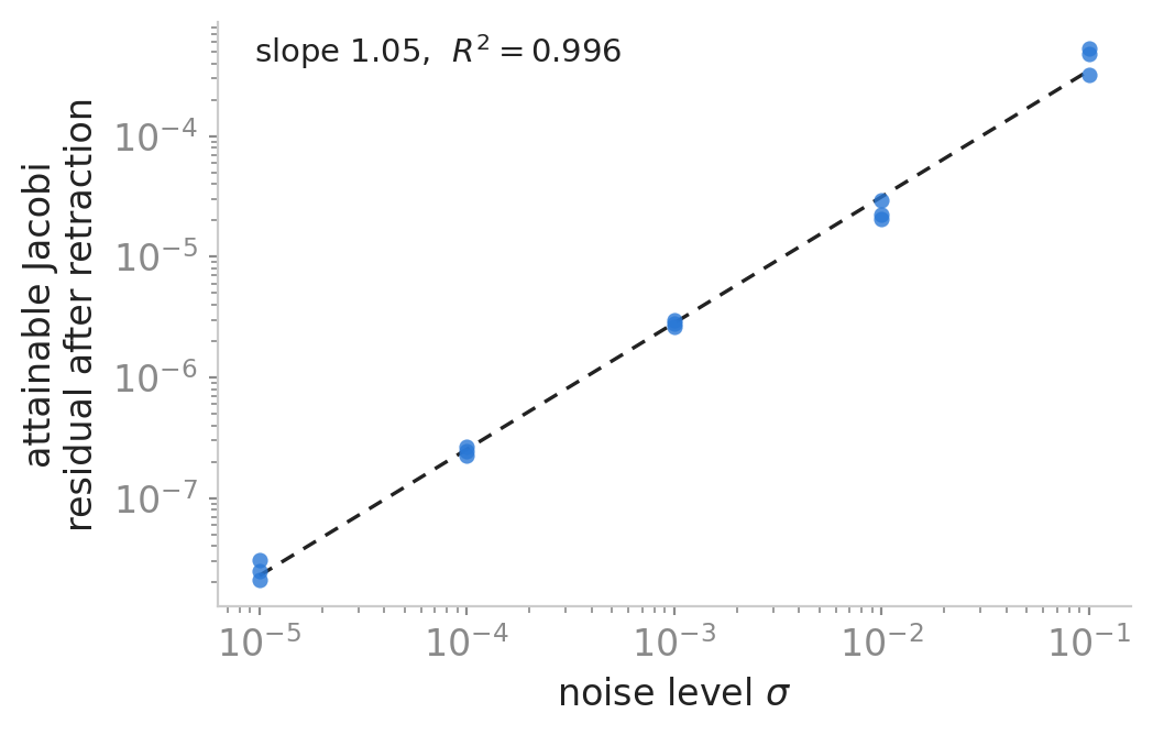
The retraction moves only where the data are silent. On the certified grid it lifts the $c$-cosine from the ceiling $0.2625$ to $1.0000$ (worst cell $0.99992$) and leaves the quotient error at $0.00705$, unchanged to every digit reported. The Jacobi residual improves from $5.3\cdot10^{-3}$ to $1.4\cdot10^{-5}$ without reaching the $10^{-16}$ of the noiseless case, and that gap is the point of the acceptance gate: under the fixed $10^{-8}$ test the automatic mode would decline the lever on all $18$ cells; under the noise-calibrated form every one is accepted.
| arm | $c$-cosine | quotient err. | steps | Jacobi cert. | gauge comp. |
|---|---|---|---|---|---|
| full-space LS | 0.2625 | 0.00705 | 1 | $5.3\cdot10^{-3}$ | $2.8\cdot10^{-15}$ |
| hook (gauge-fixed) | 0.2625 | 0.00705 | 1 | $5.3\cdot10^{-3}$ | $1.2\cdot10^{-15}$ |
| hook + retraction | 1.0000 | 0.00705 | 10 | $1.4\cdot10^{-5}$ | 0.965 |
| soft Jacobi penalty | 1.0000 | 0.00110 | 609 | $8.0\cdot10^{-7}$ | 0.965 |
Table 4. Components at matched budget under observation noise; medians over the 18 cells of the certified grid. The quotient error is what the data determine; the $c$-cosine is what the gauge hides; “gauge component” is the fraction of the estimate's displacement lying inside $K_A$.
Noisy states move the design matrix itself, so the least-squares estimate is biased. What cannot move is structural, the invisible subspace being a function of the dimension and the Hessian alone: across $27$ cells the measured nullity of the design built from noisy states is the predicted $\binom83$ at every noise level. What degrades is the budget rule's constant, in the optimistic direction, by a median factor of $1.6$ to $1.7$ when the two noise levels are matched up to $10^{-2}$, by $5.2$ when matched at $10^{-1}$, and by $533$ when state noise dominates the fields; treat the rule as a lower bound there. Total least squares does not repair it. The pipeline does not return a wrong bracket quietly: the cosine after retraction stays at $1.0000$ through state noise $10^{-2}$, and every cell where it falls is refused by the acceptance gate.
Handing the whole procedure a wrong Hessian, and never correcting it, costs accuracy but not safety, and the safety is almost entirely refusal: over $108$ cells spanning $\delta$ up to $10^{-1}$ the certificate accepts three, all at $\delta=0$, all at cosine $1.0000$. Nothing below cosine $0.99$ is certified because under a misspecified energy nearly nothing is certified at all. The residual says the rest without ground truth: for $\delta\ge10^{-3}$ it is proportional to $\delta$ with a constant between $1.2$ and $1.6$. A residual an order above the noise floor is a misspecified energy, not a missing lever.
Predicting the budget
Quotienting the gauge leaves the reduced design at full column rank, so the Gauss–Markov identity applies as written. The noise amplification $\sum_i s_i^{-2}$, over the singular values $s_i$ of that design, is computable from a pilot orbit before the fitting data are collected, so $K^\ast$ is predicted rather than searched. Over the $108$ noisy cells on $\mathfrak{so}(3)$ and $\mathfrak{su}(3)$, $100$ of them unsaturated and entering the fit, a pooled log-log fit of the error against $\sigma/s_{\min}$ has slope $1.019$ with $R^2=0.9885$. The fitted constant has median $1.78$, IQR $[1.45,2.09]$; the sharp form's prediction deviates from the measured error by $3.2\%$ in the median and at most $24\%$. Finite-difference truncation, substituted for observation noise, obeys the same scaling with slope $0.755$ but a design-correlated constant of median $7.0$: use the finite-difference row as a scaling with an $O(10)$ constant, never as a prediction.
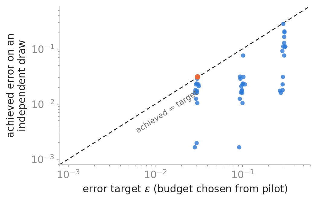
The three components run as one procedure: certify, predict the orbit budget $K^\ast$ from the quotient margin, collect that many orbits, fit on the quotient, retract, and report the quotient error and the certificate. Nothing in the loop is tuned against the answer. On $\mathfrak{su}(3)$ over $\varepsilon\in\{0.1,0.03,0.01\}$ crossed with $\sigma_{\mathrm{rel}}\in\{10^{-3},10^{-2}\}$ and three seeds, all $18$ cells land at or under the target $\varepsilon$ at the predicted budget, with $K^\ast\in\{8,16,32\}$, and no cell reaches the refusal path. Empirical against predicted $K^\ast$ agree in $32$ of $32$ cells, two by agreeing to refuse.
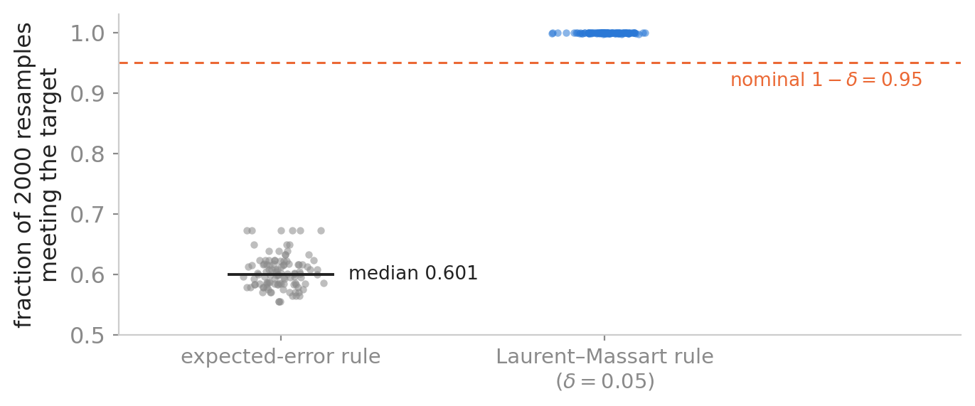
The orbit budget carries a guarantee. Over the budget ladder's 108 noisy cells resampled 2000 times each, the mean-based budget is met on a median 0.601 of draws; the $1-\delta$ bound at $\delta=0.05$ is met on at least 0.997 in every cell. The budget ladder quantises, so the guarantee costs little: the $1-\delta$ budget takes the same rung as the mean in 12 of 24 cells and one rung higher in 7; it refuses in 3 where the mean-based rule still returns a budget, and 2 further cells refuse under both rules. When the budget is chosen from pilot orbits and the fit is then made on an independent draw of initial conditions, over 45 cells one refuses and 43 of the remaining 44 meet their target, with the achieved error at 0.32 of target in the median and the single miss overshooting by 5%.
A dimension-aware Jacobi gate
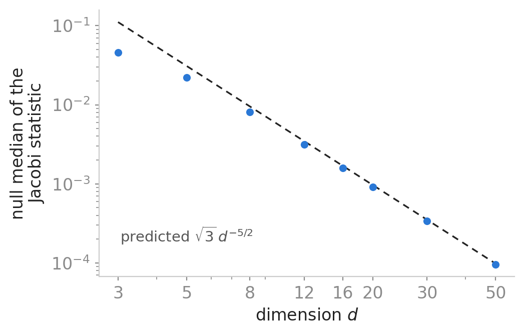
How small must a Jacobi residual be before it counts as evidence? The certificate's null distribution, its value on antisymmetric arrays that are not brackets, shrinks with $d$, so a tolerance fixed at $10^{-3}$ rejects every random tensor through $d=16$, where the null median is $1.58\cdot10^{-3}$, and accepts every one from $d=20$, where it is $9.15\cdot10^{-4}$: it has stopped being a test. The implemented gate is therefore dimension-aware, $\Jstat(c)<\alpha\sqrt3\,d^{-5/2}$ with $\alpha=10^{-3}$, and on a $28$-row battery it classifies correctly all $22$ rows carrying a ground-truth label, including the nine at $d\ge20$ the fixed gate wrongly accepts. The null median follows $\sqrt3\,d^{-5/2}$, fitted to these measurements rather than derived: the measured median approaches it monotonically from $0.41$ of it at $d=3$ to $0.98$ at $d=50$, with a fitted tail exponent of $-2.4463$ for $d\ge12$ against the predicted $-2.5$.
Passing it does not mean the algebra is right: $\mathfrak{sl}(2,\R)$ and $\mathfrak{se}(2)$ satisfy the Jacobi identity by construction and are separated from $\mathfrak{so}(3)$ only by the Killing form, at signature distances of $2.549$ and $1.414$ against $0$. A random tensor driven onto the variety by gradient descent also passes, its residual at $6.7\cdot10^{-4}$ of the random-tensor null median, and carries a rank-one Killing form at distance $2.449$. The Killing data separate every Jacobi passer in that battery while keeping two gauge copies of $\mathfrak{so}(3)$ together with it at distances $7.5\cdot10^{-10}$ and $0$. A Jacobi certificate is a necessary condition and should be reported alongside an isomorphism-class invariant, never alone.
Failure modes
The method, and the diagnostics one would naturally use to check it, can report success while being wrong. The catalog below lists nine such modes, each with a measured symptom and the mitigation the reference implementation ships.
| failure mode | measured symptom | mitigation | |
|---|---|---|---|
| F1 | float32 structure constants inflate numerical rank |
At $d=8$ the certificate reads $8.6\cdot10^{-11}$ instead of $1.1\cdot10^{-18}$; $\dim Z^2$ is reported as 19 instead of 56 and $\rJac$ as 9 instead of 21 | Raise on sub-float64 input instead of upcasting it silently |
| F2 | Fixed Jacobi tolerance at high $d$ | The $10^{-3}$ gate accepts random tensors from $d=20$; acceptance rate flips $0\to1$ | Dimension-aware gate $\alpha\sqrt3\,d^{-5/2}$ |
| F3 | Certified Jacobi, wrong algebra | Five battery rows: field agrees to $7.7\cdot10^{-15}$, Jacobi residual $\le1.2\cdot10^{-16}$, and the $GL(d)$-invariants differ | Report $\iota_H$ before fitting; report an isomorphism-class invariant beside the residual, never the residual alone |
| F4 | Small-$K$ margin is a random variable | $\mathfrak{su}(3)$ at $K\le4$: the margin spans $1.2\cdot10^{-4}$ to $1.7\cdot10^{-3}$ across seeds and is non-monotone in $K$ | Compute $K^\ast$ from the realized pilot design; treat $K^\ast\le4$ as provisional |
| F5 | Saturation: the estimate is worse than returning zero | $\mathfrak{su}(3)$, $K=2$, $\sigma_{\rm rel}=0.1$: relative error 5.57 against a predicted 4.35; the rule holds, the estimate is useless; 8 of 108 noisy cells | Refuse when $\sigma\sqrt{\sum_i s_i^{-2}}\gtrsim\|u^\ast\|$, and report the refusal instead of a number |
| F6 | Degenerate orbits give a structural, not a statistical, wall | Cubic energy with all initial conditions on one sphere: excess nullity 63–140 at $K=1$; zero excess only from $K=16$ | Spread the orbit radii; check the design's nullity against $\binom d3$ at a strict tolerance |
| F7 | A near-degenerate pilot orbit voids the a priori budget | $\mathfrak{so}(3)$, $K=1$, one seed in five: margin $3.3\cdot10^{-8}$, predicted error $2.7\cdot10^{-3}$ against an achieved $3.9\cdot10^{-7}$ | Draw the pilot from more than one orbit; reject outlier-margin pilots |
| F8 | Check C1 used as a construction step rather than as a test | Projecting the tested direction off $B^2$ takes it out of $K_A$: field difference $7.7\cdot10^{-1}$ where invisibility needs $10^{-15}$ | Use the component off $B^2$ only as a test; keep the direction inside the intersection |
| F9 | numpy.linalg.qr used for an orthonormal basis of a column space |
$B^2$ is $9\times9$ of rank 6 at $d=3$, so the reduced $Q$ spans the ambient space and the fraction outside $B^2$ reads 0.000 on rows where $\iota_H=1$ | Take orthonormal bases of column spaces by SVD, with an explicit rank tolerance |
Table 5. Failure-mode catalog: each row is a way the method or one of its diagnostics can mislead, the measured symptom, and the mitigation applied in the reference implementation.
A decision procedure
- Compute the ambiguity first. From the state dimension alone, $\binom{d}{3}$ coefficients are invisible under a single quadratic energy; for several planned energies, Theorem 2 counts what survives all of them.
- Decide whether the coefficients are the deliverable. For prediction, rollout or control synthesis the ambiguity is harmless, every member of the quotient class generating the same trajectories. What follows applies when the constants themselves are the object.
- Certify before collecting. For a hypothesized bracket and the planned energy, compute $r_{\mathrm{Jac}}=\dim(Z^2\cap K_A)$ and $\iota_H$: one nullspace, one rank and one subspace intersection — $0.091$ s at $d=8$ and $33.3$ s at $d=16$ on one CPU core.
- If $r_{\mathrm{Jac}}=0$, use the Jacobi lever. The truth is isolated in its invisible coset, so fitting in the quotient and retracting recovers it without disturbing what the data determined. Without ground truth the test is $r_{\mathrm{Jac}}$ re-read at the retracted candidate, and the procedure refuses where that reading is not decisive.
- If $r_{\mathrm{Jac}}>0$, change the experiment, not the sample size. The surviving directions stay on the Lie variety, so Jacobi enforcement cannot choose among them, and $\iota_H$ says what the ambiguity costs: a change of basis when $\iota_H=0$, a non-isomorphic algebra when $\iota_H>0$. The lever is a second energy with pairwise-distinct curvature ratios.
- Predict the budget. Quotienting makes the design full rank, so the parameter error obeys the Gauss–Markov trace $\sigma^2\sum_i s_i^{-2}$ with equality and one pilot orbit fixes the orbit count for a target accuracy; its refusal branch is informative. Under finite-difference fields the rule is a scaling with an $O(10)$ constant, never a prediction.
What is proved, what is measured
| claim | standing | scope |
|---|---|---|
| $\ker\Phi_A=0\oplus\KA$ | exact | $A$ symmetric, corank $\le1$ |
| forced ceiling | exact | noiseless, min-norm estimate |
| $\rJacExt\le\rJac$ | exact | every compatible $J_0$ |
| its Jacobi block | first order | over-counts the tangent cone |
| finite displacement | exact | a criterion, not a tolerance |
| stability of the count | exact | needs the measured gap |
| $1-\delta$ budget | exact | Gaussian noise; coverage $\ge0.997$ |
| $\rJac=\tfrac{d(d-3)}2+\nu$ | exact | compact semisimple, $A=I$ |
| $\rJacExt=3$ at $\mathfrak{su}(3)$ | generic | rises to $5,7$ on two strata |
| median $\Jstat\sim\sqrt3\,d^{-5/2}$ | fitted | $3\le d\le50$ |
| acceptance gate | calibrated | four decades of $\sigma$ |
Table 6. The standing of each claim. Exact holds identically; first order holds on the tangent cone and may fail at finite displacement; fitted is a regression over a stated range, carrying no asymptotic claim; generic holds off a measure-zero set of the stated parameter; calibrated means the threshold is set from the measured null over the stated range.
Cost and software
Everything runs on one laptop CPU core with no GPU and no training loop, the full battery in $67$ s. Two stages dominate, the certificate nullspace and the Levenberg–Marquardt normal matrix, both $\Theta(d^{10})$ in time and $\Theta(d^7)$ in memory. In float64 on one CPU core the certificate nullspace costs $0.091$ s at $d=8$ and $33.3$ s at $d=16$; end-to-end recovery on $\mathfrak{su}(3)$ with $16$ orbits returns in $0.21$ s. The binding limit is memory: the certificate matrix occupies $7.3$ MB at $d=8$, $1.01$ GB at $d=16$ and $17.6$ GB at $d=24$, so dense factorization is comfortable to $d\approx16$ and impractical beyond $d\approx20$.
The procedure is a single NumPy module of 410 lines with two entry points. From $d$, an
energy model and an optional candidate bracket, certify returns the gauge dimension
and basis, the quotient basis, $\iotaH$, the cosine ceiling of Corollary 1, the lever, and
a callable returning $K^\ast$ and its predicted error or a refusal. discover
returns $\hat c$, $\hat J_0$, the lever used, the Jacobi residual, the quotient cosine bound,
the pre-retraction estimate and the retraction trace, routing by default from the certificate at
the retracted candidate so no ground truth is required. The test suite is eighteen cases in a
few seconds, and the thirteen-algebra battery reproduces bit for bit on rerun. Beside the module
and suite, the archive carries one short producer script per experiment; each writes a
machine-readable results file, and every number printed here is transcribed from one.
Limitations
The scope is affine brackets with quadratic energies.
Confinement to $\KA$ makes the retraction's guarantee unconditional and, under noise, costs accuracy: the Jacobi identity constrains the identifiable component too, so a method free to move that component can correct part of the noise in it. A soft penalty at $\lambda\in[10^2,10^3]$ does exactly that, matching the retraction's cosine at a quotient error six times smaller. Where that component is wanted as accurately as possible and no unconditional guarantee is needed, it is the better arm.
The certificate is one-sided: $\iotaH>0$ does not by itself produce a competing algebra, which is why the five impersonation rows are exhibited directly. The first-order proposition is about tangent cones: where the intersection is positive the finite-displacement conclusion is verified numerically along an explicit line rather than proved.
The budget rule is derived for Gaussian noise on observed fields with exact states and gradients, and finite-difference truncation transfers it in shape but not in constant. With the states noisy too the rule survives as an order of magnitude rather than an identity, optimistic by a median factor of $1.6$ to $1.7$ at matched noise up to $10^{-2}$ and by $5.2$ at $10^{-1}$; it should be read as a lower bound there.
Throughout, the energy Hessian $A$ is treated as known without error: the gauge, the certificate and the retraction direction all condition on it. As a first sensitivity measurement we replace $A$ by $A+\delta\|A\|_2\,\mathrm{sym}(G)$ with $G$ Gaussian, $\delta$ up to $10^{-1}$: this leaves the three integers (gauge dimension, $\rJac$, $\iotaH$) unchanged in all $72$ cells on $\mathfrak{so}(3)$ and $\mathfrak{su}(3)$, while the ceiling moves continuously, by at most $1.7\,\delta$ across the sweep. Isolation, where it holds, is local at the truth, while the retraction starts a full coset displacement away: no basin guarantee is given, and re-evaluating the certificate at the retracted candidate is only a check after the fact.
Beyond $d\approx20$ the certificate needs a structured or randomized nullspace method, not developed here. And what these results leave open is the behavior at higher bracket degree: a cubic energy removed the kernel at bracket degree one in the cases measured, but for a bracket of higher degree $q$ the ambiguity is expected to migrate to degree $q-1$, where neither the dimension count nor the certificate has been established.
BibTeX
@misc{kandukoori2026samedynamics,
  title  = {Same Dynamics, Different Structures in Energy-Preserving Operator Fits},
  author = {Kandukoori, Sushaan and Patel, Aarya},
  year   = {2026},
  note   = {Preprint}
}